Matlab colorbar with Gnuplot

This time another colormap plot. If you are using Matlab or Octave you are probably be familiar with Matlabs nice default colormap jet.

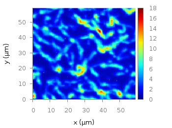
Fig. 1 Photoluminescence yield plotted with the jet colormap from Matlab (code to produce this figure, data)

In Fig.1, you see a photoluminescence yield in a given region, and as you can see Gnuplot is able to apply the jet colormap from Matlab. This can be achieved by defining the palette as follows.

set palette defined ( 0 '#000090',\
                      1 '#000fff',\
                      2 '#0090ff',\
                      3 '#0fffee',\
                      4 '#90ff70',\
                      5 '#ffee00',\
                      6 '#ff7000',\
                      7 '#ee0000',\
                      8 '#7f0000')

The numbers 0..8 are automatically rescaled to 0..1, which means you can employ arbitrary numbers here, only their difference counts.

If you want to use this colormap regularly, you can store it in the Gnuplot config file as a macro.

# ~/.gnuplot
set macros
MATLAB = "defined (0  0.0 0.0 0.5, \
                   1  0.0 0.0 1.0, \
                   2  0.0 0.5 1.0, \
                   3  0.0 1.0 1.0, \
                   4  0.5 1.0 0.5, \
                   5  1.0 1.0 0.0, \
                   6  1.0 0.5 0.0, \
                   7  1.0 0.0 0.0, \
                   8  0.5 0.0 0.0 )"

Here we defined the colors directly as rgb values in the range of 0..1, which can be alternatively used a color definition.
In order to apply the colormap, we now can simple write

set palette @MATLAB